Data Warehouse Definition
Different people have different definitions for a data warehouse. The most popular definition came from Bill Inmon, who provided the following:
A data warehouse is a subject-oriented, integrated, time-variant and non-volatile collection of data in support of management's decision making process.
Subject-Oriented: A data warehouse can be used to analyze a particular subject area. For example, "sales" can be a particular subject.
Integrated: A data warehouse integrates data from multiple data sources. For example, source A and source B may have different ways of identifying a product, but in a data warehouse, there will be only a single way of identifying a product.
Time-Variant: Historical data is kept in a data warehouse. For example, one can retrieve data from 3 months, 6 months, 12 months, or even older data from a data warehouse. This contrasts with a transactions system, where often only the most recent data is kept. For example, a transaction system may hold the most recent address of a customer, where a data warehouse can hold all addresses associated with a customer.
Non-volatile: Once data is in the data warehouse, it will not change. So, historical data in a data warehouse should never be altered.
Ralph Kimball provided a more concise definition of a data warehouse:
A data warehouse is a copy of transaction data specifically structured for query and analysis.
This is a functional view of a data warehouse. Kimball did not address how the data warehouse is built like Inmon did; rather he focused on the functionality of a data warehouse.
Data Warehouse Architecture
Different data warehousing systems have different structures. Some may have an ODS (operational data store), while some may have multiple data marts. Some may have a small number of data sources, while some may have dozens of data sources. In view of this, it is far more reasonable to present the different layers of a data warehouse architecture rather than discussing the specifics of any one system.
In general, all data warehouse systems have the following layers:
The picture below shows the relationships among the different components of the data warehouse architecture:

Each component is discussed individually below:
Data Source Layer
This represents the different data sources that feed data into the data warehouse. The data source can be of any format -- plain text file, relational database, other types of database, Excel file, etc., can all act as a data source.
Many different types of data can be a data source:
Third-party data, such as census data, demographics data, or survey data.
All these data sources together form the Data Source Layer.
Data Extraction Layer
Data gets pulled from the data source into the data warehouse system. There is likely some minimal data cleansing, but there is unlikely any major data transformation.
Staging Area
This is where data sits prior to being scrubbed and transformed into a data warehouse / data mart. Having one common area makes it easier for subsequent data processing / integration.
ETL Layer
This is where data gains its "intelligence", as logic is applied to transform the data from a transactional nature to an analytical nature. This layer is also where data cleansing happens. The ETL design phase is often the most time-consuming phase in a data warehousing project, and an ETL tool is often used in this layer.
Data Storage Layer
This is where the transformed and cleansed data sit. Based on scope and functionality, 3 types of entities can be found here: data warehouse, data mart, and operational data store (ODS). In any given system, you may have just one of the three, two of the three, or all three types.
Data Logic Layer
This is where business rules are stored. Business rules stored here do not affect the underlying data transformation rules, but do affect what the report looks like.
Data Presentation Layer
This refers to the information that reaches the users. This can be in a form of a tabular / graphical report in a browser, an emailed report that gets automatically generated and sent everyday, or an alert that warns users of exceptions, among others. Usually an OLAP tool and/or a reporting tool is used in this layer.
Metadata Layer
This is where information about the data stored in the data warehouse system is stored. A logical data model would be an example of something that's in the metadata layer. A metadata tool is often used to manage metadata.
System Operations Layer
This layer includes information on how the data warehouse system operates, such as ETL job status, system performance, and user access history.
Data Warehousing Concepts
Several concepts are of particular importance to data warehousing. They are discussed in detail in this section.
Dimensional Data Model: Dimensional data model is commonly used in data warehousing systems. This section describes this modeling technique, and the two common schema types, star schema and snowflake schema.
Slowly Changing Dimension: This is a common issue facing data warehousing practioners. This section explains the problem, and describes the three ways of handling this problem with examples.
Conceptual Data Model: What is a conceptual data model, its features, and an example of this type of data model.
Logical Data Model: What is a logical data model, its features, and an example of this type of data model.
Physical Data Model: What is a physical data model, its features, and an example of this type of data model.
Conceptual, Logical, and Physical Data Model: Different levels of abstraction for a data model. This section compares and contrasts the three different types of data models.
Data Integrity: What is data integrity and how it is enforced in data warehousing.
What is OLAP: Definition of OLAP.
MOLAP, ROLAP, and HOLAP: What are these different types of OLAP technology? This section discusses how they are different from the other, and the advantages and disadvantages of each.
Bill Inmon vs. Ralph Kimball: These two data warehousing heavyweights have a different view of the role between data warehouse and data mart.
Factless Fact Table: A fact table without any fact may sound silly, but there are real life instances when a factless fact table is useful in data warehousing.
Junk Dimension: Discusses the concept of a junk dimension: When to use it and why is it useful.
Conformed Dimension: Discusses the concept of a conformed dimension: What is it and why is it important.
Dimensional Data Model
Dimensional data model is most often used in data warehousing systems. This is different from the 3rd normal form, commonly used for transactional (OLTP) type systems. As you can imagine, the same data would then be stored differently in a dimensional model than in a 3rd normal form model.
To understand dimensional data modeling, let's define some of the terms commonly used in this type of modeling:
Dimension: A category of information. For example, the time dimension.
Attribute: A unique level within a dimension. For example, Month is an attribute in the Time Dimension.
Hierarchy: The specification of levels that represents relationship between different attributes within a dimension. For example, one possible hierarchy in the Time dimension is Year → Quarter → Month → Day.
Fact Table: A fact table is a table that contains the measures of interest. For example, sales amount would be such a measure. This measure is stored in the fact table with the appropriate granularity. For example, it can be sales amount by store by day. In this case, the fact table would contain three columns: A date column, a store column, and a sales amount column.
Lookup Table: The lookup table provides the detailed information about the attributes. For example, the lookup table for the Quarter attribute would include a list of all of the quarters available in the data warehouse. Each row (each quarter) may have several fields, one for the unique ID that identifies the quarter, and one or more additional fields that specifies how that particular quarter is represented on a report (for example, first quarter of 2001 may be represented as "Q1 2001" or "2001 Q1").
A dimensional model includes fact tables and lookup tables. Fact tables connect to one or more lookup tables, but fact tables do not have direct relationships to one another. Dimensions and hierarchies are represented by lookup tables. Attributes are the non-key columns in the lookup tables.
In designing data models for data warehouses / data marts, the most commonly used schema types are Star Schema and Snowflake Schema.
Whether one uses a star or a snowflake largely depends on personal preference and business needs. Personally, I am partial to snowflakes,when there is a business case to analyze the information at that particular level.
Star Schema
In the star schema design, a single object (the fact table) sits in the middle and is radically connected to other surrounding objects (dimension lookup tables) like a star. Each dimension is represented as a single table. The primary key in each dimension table is related to a foreign key in the fact table.
Sample star schema
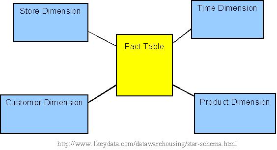
All measures in the fact table are related to all the dimensions that fact table is related to. In other words, they all have the same level of granularity.
A star schema can be simple or complex. A simple star consists of one fact table; a complex star can have more than one fact table.
Let's look at an example: Assume our data warehouse keeps store sales data, and the different dimensions are time, store, product, and customer. In this case, the figure on the left represents our star schema. The lines between two tables indicate that there is a primary key / foreign key relationship between the two tables. Note that different dimensions are not related to one another.
Snowflake Schema
The snowflake schema is an extension of the star schema, where each point of the star explodes into more points. In a star schema, each dimension is represented by a single dimensional table, whereas in a snowflake schema, that dimensional table is normalized into multiple lookup tables, each representing a level in the dimensional hierarchy.
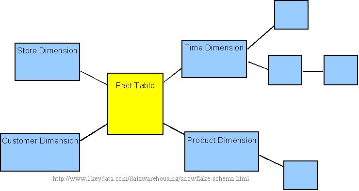
For example, the Time Dimension that consists of 2 different hierarchies:
1. Year → Month → Day
2. Week → Day
We will have 4 lookup tables in a snowflake schema: A lookup table for year, a lookup table for month, a lookup table for week, and a lookup table for day. Year is connected to Month, which is then connected to Day. Week is only connected to Day. A sample snowflake schema illustrating the above relationships in the Time Dimension is shown to the right.
The main advantage of the snowflake schema is the improvement in query performance due to minimized disk storage requirements and joining smaller lookup tables. The main disadvantage of the snowflake schema is the additional maintenance efforts needed due to the increase number of lookup tables.
Fact Table Granularity
Granularity
The first step in designing a fact table is to determine the granularity of the fact table. By granularity, we mean the lowest level of information that will be stored in the fact table. This constitutes two steps:
- Determine which dimensions will be included.
- Determine where along the hierarchy of each dimension the information will be kept.
The determining factors usually goes back to the requirements.
Which Dimensions To Include
Determining which dimensions to include is usually a straightforward process, because business processes will often dictate clearly what are the relevant dimensions.
For example, in an off-line retail world, the dimensions for a sales fact table are usually time, geography, and product. This list, however, is by no means a complete list for all off-line retailers. A supermarket with a Rewards Card program, where customers provide some personal information in exchange for a rewards card, and the supermarket would offer lower prices for certain items for customers who present a rewards card at checkout, will also have the ability to track the customer dimension. Whether the data warehousing system includes the customer dimension will then be a decision that needs to be made.
What Level Within Each Dimension To Include
Determining which part of hierarchy the information is stored along each dimension is not an exact science. This is where user requirement (both stated and possibly future) plays a major role.
In the above example, will the supermarket wanting to do analysis along at the hourly level? (i.e., looking at how certain products may sell by different hours of the day.) If so, it makes sense to use 'hour' as the lowest level of granularity in the time dimension. If daily analysis is sufficient, then 'day' can be used as the lowest level of granularity. Since the lower the level of detail, the larger the data amount in the fact table, the granularity exercise is in essence figuring out the sweet spot in the tradeoff between detailed level of analysis and data storage.
Note that sometimes the users will not specify certain requirements, but based on the industry knowledge, the data warehousing team may foresee that certain requirements will be forthcoming that may result in the need of additional details. In such cases, it is prudent for the data warehousing team to design the fact table such that lower-level information is included. This will avoid possibly needing to re-design the fact table in the future. On the other hand, trying to anticipate all future requirements is an impossible and hence futile exercise, and the data warehousing team needs to fight the urge of the "dumping the lowest level of detail into the data warehouse" symptom, and only includes what is practically needed. Sometimes this can be more of an art than science, and prior experience will become invaluable here.
Fact And Fact Table Types
Types of Facts
There are three types of facts:
- Additive: Additive facts are facts that can be summed up through all of the dimensions in the fact table.
- Semi-Additive: Semi-additive facts are facts that can be summed up for some of the dimensions in the fact table, but not the others.
- Non-Additive: Non-additive facts are facts that cannot be summed up for any of the dimensions present in the fact table.
Let us use examples to illustrate each of the three types of facts. The first example assumes that we are a retailer, and we have a fact table with the following columns:
| Date |
| Store |
| Product |
| Sales_Amount |
The purpose of this table is to record the sales amount for each product in each store on a daily basis. Sales_Amount is the fact. In this case,Sales_Amount is an additive fact, because you can sum up this fact along any of the three dimensions present in the fact table -- date, store, and product. For example, the sum of Sales_Amount for all 7 days in a week represents the total sales amount for that week.
Say we are a bank with the following fact table:
| Date |
| Account |
| Current_Balance |
| Profit_Margin |
The purpose of this table is to record the current balance for each account at the end of each day, as well as the profit margin for each account for each day. Current_Balance and Profit_Margin are the facts. Current_Balance is a semi-additive fact, as it makes sense to add them up for all accounts (what's the total current balance for all accounts in the bank?), but it does not make sense to add them up through time (adding up all current balances for a given account for each day of the month does not give us any useful information). Profit_Margin is a non-additive fact, for it does not make sense to add them up for the account level or the day level.
Types of Fact Tables
Based on the above classifications, there are two types of fact tables:
- Cumulative: This type of fact table describes what has happened over a period of time. For example, this fact table may describe the total sales by product by store by day. The facts for this type of fact tables are mostly additive facts. The first example presented here is a cumulative fact table.
- Snapshot: This type of fact table describes the state of things in a particular instance of time, and usually includes more semi-additive and non-additive facts. The second example presented here is a snapshot fact table.
Slowly Changing Dimensions
The "Slowly Changing Dimension" problem is a common one particular to data warehousing. In a nutshell, this applies to cases where the attribute for a record varies over time. We give an example below:
Christina is a customer with ABC Inc. She first lived in Chicago, Illinois. So, the original entry in the customer lookup table has the following record:
| Customer Key | Name | State |
| 1001 | Christina | Illinois |
At a later date, she moved to Los Angeles, California on January, 2003. How should ABC Inc. now modify its customer table to reflect this change? This is the "Slowly Changing Dimension" problem.
There are in general three ways to solve this type of problem, and they are categorized as follows:
Type 1: The new record replaces the original record. No trace of the old record exists.
Type 2: A new record is added into the customer dimension table. Therefore, the customer is treated essentially as two people.
Type 3: The original record is modified to reflect the change.
We next take a look at each of the scenarios and how the data model and the data looks like for each of them. Finally, we compare and contrast among the three alternatives.
Type 1 Slowly Changing Dimension
In Type 1 Slowly Changing Dimension, the new information simply overwrites the original information. In other words, no history is kept.
In our example, recall we originally have the following table:
| Customer Key | Name | State |
| 1001 | Christina | Illinois |
After Christina moved from Illinois to California, the new information replaces the new record, and we have the following table:
| Customer Key | Name | State |
| 1001 | Christina | California |
Advantages:
- This is the easiest way to handle the Slowly Changing Dimension problem, since there is no need to keep track of the old information.
Disadvantages:
- All history is lost. By applying this methodology, it is not possible to trace back in history. For example, in this case, the company would not be able to know that Christina lived in Illinois before.
Usage:
About 50% of the time.
When to use Type 1:
Type 1 slowly changing dimension should be used when it is not necessary for the data warehouse to keep track of historical changes.
Type 2 Slowly Changing Dimension
In Type 2 Slowly Changing Dimension, a new record is added to the table to represent the new information. Therefore, both the original and the new record will be present. The new record gets its own primary key.
In our example, recall we originally have the following table:
| Customer Key | Name | State |
| 1001 | Christina | Illinois |
After Christina moved from Illinois to California, we add the new information as a new row into the table:
| Customer Key | Name | State |
| 1001 | Christina | Illinois |
| 1005 | Christina | California |
Advantages:
- This allows us to accurately keep all historical information.
Disadvantages:
- This will cause the size of the table to grow fast. In cases where the number of rows for the table is very high to start with, storage and performance can become a concern.
- This necessarily complicates the ETL process.
Usage:
About 50% of the time.
When to use Type 2:
Type 2 slowly changing dimension should be used when it is necessary for the data warehouse to track historical changes.
Type 3 Slowly Changing Dimension
In Type 3 Slowly Changing Dimension, there will be two columns to indicate the particular attribute of interest, one indicating the original value, and one indicating the current value. There will also be a column that indicates when the current value becomes active.
In our example, recall we originally have the following table:
| Customer Key | Name | State |
| 1001 | Christina | Illinois |
To accommodate Type 3 Slowly Changing Dimension, we will now have the following columns:
- Customer Key
- Name
- Original State
- Current State
- Effective Date
After Christina moved from Illinois to California, the original information gets updated, and we have the following table (assuming the effective date of change is January 15, 2003):
| Customer Key | Name | Original State | Current State | Effective Date |
| 1001 | Christina | Illinois | California | 15-JAN-2003 |
Advantages:
- This does not increase the size of the table, since new information is updated.
- This allows us to keep some part of history.
Disadvantages:
- Type 3 will not be able to keep all history where an attribute is changed more than once. For example, if Christina later moves to Texas on December 15, 2003, the California information will be lost.
Usage:
Type 3 is rarely used in actual practice.
When to use Type 3:
Type III slowly changing dimension should only be used when it is necessary for the data warehouse to track historical changes, and when such changes will only occur for a finite number of time.
Conceptual Data Model


Conceptual Data Model
A conceptual data model identifies the highest-level relationships between the different entities. Features of conceptual data model include:
- Includes the important entities and the relationships among them.
- No attribute is specified.
- No primary key is specified.
The figure below is an example of a conceptual data model.
Conceptual Data Model
From the figure above, we can see that the only information shown via the conceptual data model is the entities that describe the data and the relationships between those entities. No other information is shown through the conceptual data model.
Logical Data Model
A logical data model describes the data in as much detail as possible, without regard to how they will be physical implemented in the database. Features of a logical data model include:
- Includes all entities and relationships among them.
- All attributes for each entity are specified.
- The primary key for each entity is specified.
- Foreign keys (keys identifying the relationship between different entities) are specified.
- Normalization occurs at this level.
The steps for designing the logical data model are as follows:
- Specify primary keys for all entities.
- Find the relationships between different entities.
- Find all attributes for each entity.
- Resolve many-to-many relationships.
- Normalization.
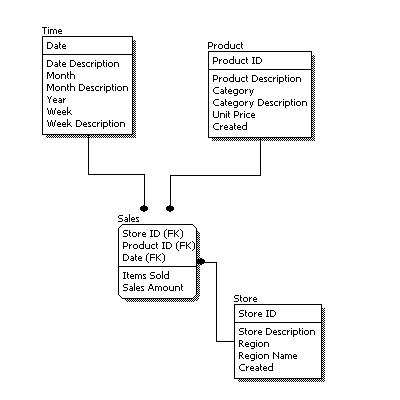
The figure below is an example of a logical data model.
Logical Data Model
Comparing the logical data model shown above with the conceptual data model diagram, we see the main differences between the two:
- In a logical data model, primary keys are present, whereas in a conceptual data model, no primary key is present.
- In a logical data model, all attributes are specified within an entity. No attributes are specified in a conceptual data model.
- Relationships between entities are specified using primary keys and foreign keys in a logical data model. In a conceptual data model, the relationships are simply stated, not specified, so we simply know that two entities are related, but we do not specify what attributes are used for this relationship.
Physical Data Model
Physical data model represents how the model will be built in the database. A physical database model shows all table structures, including column name, column data type, column constraints, primary key, foreign key, and relationships between tables. Features of a physical data model include:
- Specification all tables and columns.
- Foreign keys are used to identify relationships between tables.
- Denormalization may occur based on user requirements.
- Physical considerations may cause the physical data model to be quite different from the logical data model.
- Physical data model will be different for different RDBMS. For example, data type for a column may be different between MySQL and SQL Server.
The steps for physical data model design are as follows:
- Convert entities into tables.
- Convert relationships into foreign keys.
- Convert attributes into columns.
- Modify the physical data model based on physical constraints / requirements.
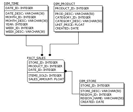
The figure below is an example of a physical data model.
Physical Data Model
Comparing the physical data model shown above with the logical data model diagram, we see the main differences between the two:
- Entity names are now table names.
- Attributes are now column names.
- Data type for each column is specified. Data types can be different depending on the actual database being used.
Data Modeling - Conceptual, Logical, And Physical Data Models
The three levels of data modeling, conceptual data model, logical data model, and physical data model, were discussed in prior sections. Here we compare these three types of data models. The table below compares the different features:
| Feature | Conceptual | Logical | Physical |
| Entity Names | |||
| Entity Relationships | |||
| Attributes | |||
| Primary Keys | |||
| Foreign Keys | |||
| Table Names | |||
| Column Names | |||
| Column Data Types |
Below we show the conceptual, logical, and physical versions of a single data model.
Conceptual Model Design | Logical Model Design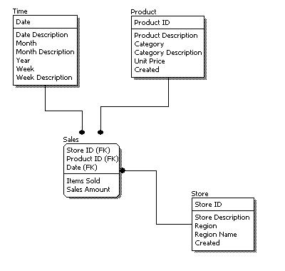 | Physical Model Design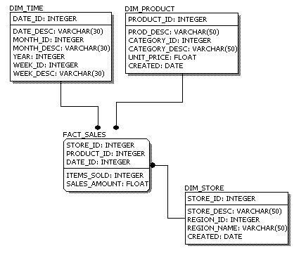 |
We can see that the complexity increases from conceptual to logical to physical. This is why we always first start with the conceptual data model (so we understand at high level what are the different entities in our data and how they relate to one another), then move on to the logical data model (so we understand the details of our data without worrying about how they will actually implemented), and finally the physical data model (so we know exactly how to implement our data model in the database of choice). In a data warehousing project, sometimes the conceptual data model and the logical data model are considered as a single deliverable.
Data Integrity
Data integrity refers to the validity of data, meaning data is consistent and correct. In the data warehousing field, we frequently hear the term, "Garbage In, Garbage Out." If there is no data integrity in the data warehouse, any resulting report and analysis will not be useful.
In a data warehouse or a data mart, there are three areas of where data integrity needs to be enforced:
Database level
We can enforce data integrity at the database level. Common ways of enforcing data integrity include:
Referential integrity
The relationship between the primary key of one table and the foreign key of another table must always be maintained. For example, a primary key cannot be deleted if there is still a foreign key that refers to this primary key.
Primary key / Unique constraint
Primary keys and the UNIQUE constraint are used to make sure every row in a table can be uniquely identified.
Not NULL vs. NULL-able
For columns identified as NOT NULL, they may not have a NULL value.
Valid Values
Only allowed values are permitted in the database. For example, if a column can only have positive integers, a value of '-1' cannot be allowed.
ETL process
For each step of the ETL process, data integrity checks should be put in place to ensure that source data is the same as the data in the destination. Most common checks include record counts or record sums.
Access level
We need to ensure that data is not altered by any unauthorized means either during the ETL process or in the data warehouse. To do this, there needs to be safeguards against unauthorized access to data (including physical access to the servers), as well as logging of all data access history. Data integrity can only ensured if there is no unauthorized access to the data.
What Is OLAP
OLAP stands for On-Line Analytical Processing. The first attempt to provide a definition to OLAP was by Dr. Codd, who proposed 12 rules for OLAP. Later, it was discovered that this particular white paper was sponsored by one of the OLAP tool vendors, thus causing it to lose objectivity. The OLAP Report has proposed the FASMI test, Fast Analysis of Shared Multidimensional Information. For a more detailed description of both Dr. Codd's rules and the FASMI test, please visit The OLAP Report.
For people on the business side, the key feature out of the above list is "Multidimensional." In other words, the ability to analyze metrics in different dimensions such as time, geography, gender, product, etc. For example, sales for the company are up. What region is most responsible for this increase? Which store in this region is most responsible for the increase? What particular product category or categories contributed the most to the increase? Answering these types of questions in order means that you are performing an OLAP analysis.
Depending on the underlying technology used, OLAP can be broadly divided into two different camps: MOLAP and ROLAP. A discussion of the different OLAP types can be found in the MOLAP, ROLAP, and HOLAP section.
MOLAP, ROLAP, And HOLAP
In the OLAP world, there are mainly two different types: Multidimensional OLAP (MOLAP) and Relational OLAP (ROLAP). Hybrid OLAP (HOLAP) refers to technologies that combine MOLAP and ROLAP.
MOLAP
This is the more traditional way of OLAP analysis. In MOLAP, data is stored in a multidimensional cube. The storage is not in the relational database, but in proprietary formats.
Advantages:
- Excellent performance: MOLAP cubes are built for fast data retrieval, and are optimal for slicing and dicing operations.
- Can perform complex calculations: All calculations have been pre-generated when the cube is created. Hence, complex calculations are not only doable, but they return quickly.
Disadvantages:
- Limited in the amount of data it can handle: Because all calculations are performed when the cube is built, it is not possible to include a large amount of data in the cube itself. This is not to say that the data in the cube cannot be derived from a large amount of data. Indeed, this is possible. But in this case, only summary-level information will be included in the cube itself.
- Requires additional investment: Cube technology are often proprietary and do not already exist in the organization. Therefore, to adopt MOLAP technology, chances are additional investments in human and capital resources are needed.
ROLAP
This methodology relies on manipulating the data stored in the relational database to give the appearance of traditional OLAP's slicing and dicing functionality. In essence, each action of slicing and dicing is equivalent to adding a "WHERE" clause in the SQL statement.
Advantages:
- Can handle large amounts of data: The data size limitation of ROLAP technology is the limitation on data size of the underlying relational database. In other words, ROLAP itself places no limitation on data amount.
- Can leverage functionalities inherent in the relational database: Often, relational database already comes with a host of functionalities. ROLAP technologies, since they sit on top of the relational database, can therefore leverage these functionalities.
Disadvantages:
- Performance can be slow: Because each ROLAP report is essentially a SQL query (or multiple SQL queries) in the relational database, the query time can be long if the underlying data size is large.
- Limited by SQL functionalities: Because ROLAP technology mainly relies on generating SQL statements to query the relational database, and SQL statements do not fit all needs (for example, it is difficult to perform complex calculations using SQL), ROLAP technologies are therefore traditionally limited by what SQL can do. ROLAP vendors have mitigated this risk by building into the tool out-of-the-box complex functions as well as the ability to allow users to define their own functions.
HOLAP
HOLAP technologies attempt to combine the advantages of MOLAP and ROLAP. For summary-type information, HOLAP leverages cube technology for faster performance. When detail information is needed, HOLAP can "drill through" from the cube into the underlying relational data.
Bill Inmon vs. Ralph Kimball
In the data warehousing field, we often hear about discussions on where a person / organization's philosophy falls into Bill Inmon's camp or into Ralph Kimball's camp. We describe below the difference between the two.
Bill Inmon's paradigm: Data warehouse is one part of the overall business intelligence system. An enterprise has one data warehouse, and data marts source their information from the data warehouse. In the data warehouse, information is stored in 3rd normal form.
Ralph Kimball's paradigm: Data warehouse is the conglomerate of all data marts within the enterprise. Information is always stored in the dimensional model.
There is no right or wrong between these two ideas, as they represent different data warehousing philosophies. In reality, the data warehouse systems in most enterprises are closer to Ralph Kimball's idea. This is because most data warehouses started out as a departmental effort, and hence they originated as a data mart. Only when more data marts are built later do they evolve into a data warehouse.
Factless Fact Table
A factless fact table is a fact table that does not have any measures. It is essentially an intersection of dimensions. On the surface, a factless fact table does not make sense, since a fact table is, after all, about facts. However, there are situations where having this kind of relationship makes sense in data warehousing.
For example, think about a record of student attendance in classes. In this case, the fact table would consist of 3 dimensions: the student dimension, the time dimension, and the class dimension. This factless fact table would look like the following:
The only measure that you can possibly attach to each combination is "1" to show the presence of that particular combination. However, adding a fact that always shows 1 is redundant because we can simply use the COUNT function in SQL to answer the same questions.
Factless fact tables offer the most flexibility in data warehouse design. For example, one can easily answer the following questions with this factless fact table:
- How many students attended a particular class on a particular day?
- How many classes on average does a student attend on a given day?
Without using a factless fact table, we will need two separate fact tables to answer the above two questions. With the above factless fact table, it becomes the only fact table that's needed.
Junk Dimension
In data warehouse design, frequently we run into a situation where there are yes/no indicator fields in the source system. Through business analysis, we know it is necessary to keep such information in the fact table. However, if keep all those indicator fields in the fact table, not only do we need to build many small dimension tables, but the amount of information stored in the fact table also increases tremendously, leading to possible performance and management issues.
Junk dimension is the way to solve this problem. In a junk dimension, we combine these indicator fields into a single dimension. This way, we'll only need to build a single dimension table, and the number of fields in the fact table, as well as the size of the fact table, can be decreased. The content in the junk dimension table is the combination of all possible values of the individual indicator fields.
Let's look at an example. Assuming that we have the following fact table:
In this example, TXN_CODE, COUPON_IND, and PREPAY_IND are all indicator fields. In this existing format, each one of them is a dimension. Using the junk dimension principle, we can combine them into a single junk dimension, resulting in the following fact table:
Note that now the number of dimensions in the fact table went from 7 to 5.
The content of the junk dimension table would look like the following:
In this case, we have 3 possible values for the TXN_CODE field, 2 possible values for the COUPON_IND field, and 2 possible values for the PREPAY_IND field. This results in a total of 3 x 2 x 2 = 12 rows for the junk dimension table.
By using a junk dimension to replace the 3 indicator fields, we have decreased the number of dimensions by 2 and also decreased the number of fields in the fact table by 2. This will result in a data warehousing environment that offer better performance as well as being easier to manage.
Conformed Dimension
A conformed dimension is a dimension that has exactly the same meaning and content when being referred from different fact tables. A conformed dimension can refer to multiple tables in multiple data marts within the same organization. For two dimension tables to be considered as conformed, they must either be identical or one must be a subset of another. There cannot be any other type of difference between the two tables. For example, two dimension tables that are exactly the same except for the primary key are not considered conformed dimensions.
Why is conformed dimension important? This goes back to the definition of data warehouse being "integrated." Integrated means that even if a particular entity had different meanings and different attributes in the source systems, there must be a single version of this entity once the data flows into the data warehouse.
The time dimension is a common conformed dimension in an organization. Usually the only rule to consider with the time dimension is whether there is a fiscal year in addition to the calendar year and the definition of a week. Fortunately, both are relatively easy to resolve. In the case of fiscal vs. calendar year, one may go with either fiscal or calendar, or an alternative is to have two separate conformed dimensions, one for fiscal year and one for calendar year. The definition of a week is also something that can be different in large organizations: Finance may use Saturday to Friday, while marketing may use Sunday to Saturday. In this case, we should decide on a definition and move on. The nice thing about the time dimension is once these rules are set, the values in the dimension table will never change. For example, October 16th will never become the 15th day in October.
Not all conformed dimensions are as easy to produce as the time dimension. An example is the customer dimension. In any organization with some history, there is a high likelihood that different customer databases exist in different parts of the organization. To achieve a conformed customer dimension means those data must be compared against each other, rules must be set, and data must be cleansed. In addition, when we are doing incremental data loads into the data warehouse, we'll need to apply the same rules to the new values to make sure we are only adding truly new customers to the customer dimension.
Building a conformed dimension also part of the process in master data management, or MDM. In MDM, one must not only make sure the master data dimensions are conformed, but that conformity needs to be brought back to the source systems.


4 comments:
Did you know that you can create short urls with LinkShrink and receive dollars for every visitor to your shortened urls.
Thanks for sharing! Really good summup.
sql server developer online training
informatica online training
data modelling online training
Data Warehousing
Post a Comment