It's All About ORACLE

Oracle - The number one Database Management System. Hope this Blog will teach a lot about oracle.

Choosing a Primary Key: Natural or Surrogate?

This post overviews strategies for assigning primary keys to a table within a relational database. In particular, it focuses on the issue of when to use natural keys and when to use surrogate keys. Some people will tell you that you should always use natural keys and others will tell you that you should always use surrogate keys. These people invariably prove to be wrong, typically they're doing little more than sharing the prejudices of their "data religion" with you. The reality is that natural and surrogate keys each have their advantages and disadvantages, and that no strategy is perfect for all situations. In other words, you need to know what you're doing if you want to get it right. This article discusses:


  • Common key terminology  
  • Strategies for assigning keys
  • Surrogate key implementation strategies
  • Tips for effective keys
  • What to do when you make the "wrong" choice


  • 1. Common Key Terminology

    Let's start by describing some common terminology pertaining to keys and then work through an example. These terms are:

    • Key. A key is one or more data attributes that uniquely identify an entity.  In a physical database a key would be formed of one or more table columns whose value(s) uniquely identifies a row within a relational table. 
    • Composite key. A key that is composed of two or more attributes. 
    • Natural key. A key that is formed of attributes that already exist in the real world.  For example, U.S. citizens are issued a Social Security Number (SSN)  that is unique to them (this isn't guaranteed to be true, but it's pretty darn close in practice).  SSN could be used as a natural key, assuming privacy laws allow it, for a Person entity (assuming the scope of your organization is limited to the U.S.). 
    • Surrogate key. A key with no business meaning.
    • Candidate key. An entity type in a logical data model will have zero or more candidate keys, also referred to simply as unique identifiers (note: some people don't believe in identifying candidate keys in LDMs, so there's no hard and fast rules). For example, if we only interact with American citizens then SSN is one candidate key for the Person entity type and the combination of name and phone number (assuming the combination is unique) is potentially a second candidate key. Both of these keys are called candidate keys because they are candidates to be chosen as the primary key, an alternate key or perhaps not even a key at all within a physical data model. 
    • Primary key. The preferred key for an entity type.
    • Alternate key. Also known as a secondary key, is another unique identifier of a row within a table. 
    • Foreign key. One or more attributes in an entity type that represents a key, either primary or secondary, in another entity type.
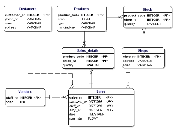
    Figure 1 presents a physical data model (PDM) for a physical address using the UML notation. In Figure 1 the Customer table has the CustomerNumber column as its primary key and SocialSecurityNumber as an alternate key. This indicates that the preferred way to access customer information is through the value of a person's customer number although your software can get at the same information if it has the person's social security number.  The CustomerHasAddress table has a composite primary key, the combination of CustomerNumber and AddressID.  A foreign key is one or more attributes in an entity type that represents a key, either primary or secondary, in another entity type.  Foreign keys are used to maintain relationships between rows.  For example, the relationships between rows in the CustomerHasAddress table and the Customer table is maintained by the CustomerNumber column within the CustomerHasAddress table. The interesting thing about the CustomerNumber column is the fact that it is part of the primary key for CustomerHasAddress as well as the foreign key to the Customer table. Similarly, theAddressID column is part of the primary key of CustomerHasAddress as well as a foreign key to the Address table to maintain the relationship with rows of Address.

    Figure 1. A simple PDM modeling Customer and Address.
      

    2. Comparing Natural and Surrogate Key Strategies

    There are two strategies for assigning keys to tables:

    1. Natural keys.  A natural key is one or more existing data attributes that are unique to the business concept.  For the Customer table there was two candidate keys, in this case CustomerNumber and SocialSecurityNumber
    2. Surrogate key. Introduce a new column, called a surrogate key, which is a key that has no business meaning. An example of which is the AddressID column of the Address table in Figure 1. Addresses don't have an "easy" natural key because you would need to use all of the columns of the Address table to form a key for itself (you might be able to get away with just the combination of Street and ZipCode depending on your problem domain), therefore introducing a surrogate key is a much better option in this case.  
    The advantage of natural keys is that they exist already, you don't need to introduce a new "unnatural" value to your data schema. However, the disadvantage of natural keys is that because they have business meaning they are effectively coupled to your business: you may need to rework your key when your business requirements change. For example, if your users decide to make CustomerNumber alphanumeric instead of numeric then in addition to updating the schema for the Customer table (which is unavoidable) you would have to change every single table whereCustomerNumber is used as a foreign key.

    There are several advantages to surrogate keys. First, they aren't coupled to your business and therefore will be easier to maintain (assuming you pick a good implementation strategy). For example, if the Customer table instead used a surrogate key then the change would have been localized to just the Customer table itself (CustomerNumber in this case would just be a non-key column of the table).  Of course, if you needed to make a similar change to your surrogate key strategy, perhaps adding a couple of extra digits to your key values because you've run out of values, then you would have the exact same problem.  Second, a common key strategy across most, or better yet all, tables can reduce the amount of source code that you need to write, reducing the total cost of ownership (TCO) of the systems that you build. The fundamental disadvantage of surrogate keys is that they're often not "human readable", making them difficult for end users to work with. The implication is that you might still need to implement alternate keys for searching, editing, and so on.
    The fundamental issue is that keys are a significant source of coupling within a relational schema, and as a result they are difficult to change. The implication is that you generally want to avoid keys with business meaning because business meaning changes. Having said that, I have a tendency to use natural keys for lookup/reference tables, particularly when I suspect that the key values won't change any time soon, as I describe below. Fundamentally, there is no clear answer as to whether or not you should prefer natural keys over surrogate keys, regardless of what the zealots on either side of this religious argument may claim, and that your best strategy is be prepared to apply one strategy or the other whenever it makes sense.

    3. Surrogate Key Implementation Strategies

    There are several common options for implementing surrogate keys:

    1. Key values assigned by the database.  Most of the leading database vendors – companies such as Oracle, Sybase, and Informix – implement a surrogate key strategy called incremental keys. The basic idea is that they maintain a counter within the database server, writing the current value to a hidden system table to maintain consistency, which they use to assign a value to newly created table rows.  Every time a row is created the counter is incremented and that value is assigned as the key value for that row.  The implementation strategies vary from vendor to vendor, sometimes the values assigned are unique across all tables whereas sometimes values are unique only within a single table, but the general concept is the same.
    2. MAX() + 1.  A common strategy is to use an integer column, start the value for the first record at 1, then for a new row set the value to the maximum value in this column plus one using the SQL MAX function.  Although this approach is simple it suffers from performance problems with large tables and only guarantees a unique key value within the table.  
    3. Universally unique identifiers (UUIDs).  UUIDs are 128-bit values that are created from a hash of the ID of your Ethernet card, or an equivalent software representation, and the current datetime of your computer system.  The algorithm for doing this is defined by the Open Software Foundation (www.opengroup.org).
    4. Globally unique identifiers (GUIDs)GUIDs are a Microsoft standard that extend UUIDs, following the same strategy if an Ethernet card exists and if not then they hash a software ID and the current datetime to produce a value that is guaranteed unique to the machine that creates it. 
    5. High-low strategy.  The basic idea is that your key value, often called a persistent object identifier (POID) or simply an object identified (OID), is in two logical parts: A unique HIGH value that you obtain from a defined source and an N-digit LOW value that your application assigns itself.  Each time that a HIGH value is obtained the LOW value will be set to zero. For example, if the application that you're running requests a value for HIGH it will be assigned the value 1701. Assuming that N, the number of digits for LOW, is four then all persistent object identifiers that the application assigns to objects will be combination of 17010000,17010001, 17010002, and so on until 17019999.  At this point a new value for HIGH is obtained, LOW is reset to zero, and you continue again. If another application requests a value for HIGH immediately after you it will given the value of 1702, and the OIDs that will be assigned to objects that it creates will be 17020000, 17020001, and so on.   As you can see, as long as HIGH is unique then all POID values will be unique.
    The fundamental issue is that keys are a significant source of coupling within a relational schema, and as a result they prove difficult to refactor. The implication is that you want to avoid keys with business meaning because business meaning changes. However, at the same time you need to remember that some data is commonly accessed by unique identifiers, for example customer via their customer number and American employees via their Social Security Number (SSN).  In these cases you may want to use the natural key instead of a surrogate key such as a UUID or POID.    

    4. Tips for Effective Keys

    How can you be effective at assigning keys?  Consider the following tips:
    1. Avoid "smart" keys.  A "smart" key is one that contains one or more subparts which provide meaning.  For example the first two digits of an U.S. zip code indicate the state that the zip code is in. The first problem with smart keys is that have business meaning.  The second problem is that their use often becomes convoluted over time. For example some large states have several codes, California has zip codes beginning with 90 and 91, making queries based on state codes more complex.  Third, they often increase the chance that the strategy will need to be expanded.  Considering that zip codes are nine digits in length (the following four digits are used at the discretion of owners of buildings uniquely identified by zip codes) it's far less likely that you'd run out of nine-digit numbers before running out of two digit codes assigned to individual states.
    2. Consider assigning natural keys for simple "look up" tables. A "look up" table is one that is used to relate codes to detailed information. For example, you might have a look up table listing color codes to the names of colors. For example the code 127 represents "Tulip Yellow". Simple look up tables typically consist of a code column and a description/name column whereas complex look up tables consist of a code column and several informational columns. 
    3. Natural keys don't always work for "look up" tables. Another example of a look up table is one that contains a row for each state, province, or territory in North America.  For example there would be a row for California, a US state, and for Ontario, a Canadian province. The primary goal of this table is to provide an official list of these geographical entities, a list that is reasonably static over time (the last change to it would have been in the late 1990s when the Northwest Territories, a territory of Canada, was split into Nunavut and Northwest Territories). A valid natural key for this table would be the state code, a unique two character code – e.g. CA for California and ON for Ontario.  Unfortunately this approach doesn't work because Canadian government decided to keep the same state code, NW, for the two territories.
    4. Your applications must still support "natural key searches". If you choose to take a surrogate key approach to your database design you mustn't forget that your applications must still support searches on the domain columns that still uniquely identify rows.  For example, your Customer table may have a Customer_POID column used as a surrogate key as well as a Customer_Number column and a Social_Security_Number column.  You would likely need to support searches based on both the customer number and the social security number.  Searching is discussed in detail in Best Practices for Retrieving Objects from a Relational Database.
    5. Don't naturalize surrogate keys. As soon as you display the value of a surrogate key to your end users, or worse yet allow them to work with the value (perhaps to search), you have effectively given the key business meaning. This in effect naturalizes the key and thereby negates some of the advantages of surrogate keys.

    5. What to Do When You Make the "Wrong" Choice

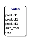
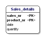
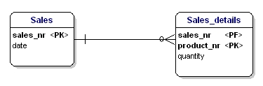
    First of all, don't worry about this: You're only human, and no matter how good you are at database design you're going to make mistakes. The good news is that as I show in The Process of Database Refactoring it is possible, albeit it may require a bit of work, to replace a natural key with a surrogate key (or vice versa). To replace a natural key with a surrogate you would apply the Introduce Surrogate Key refactoring, as you see depicted in Figure 2 to replace the key of the Order table. To replace a surrogate key with a natural key you would apply the Replace Surrogate Key with Natural Key refactoring, as you see in Figure 3 to replace the key of the State table.

    Figure 2. Replacing the natural key of the Order table.

    Figure 3. Replacing the surrogate key within the State table.

    http://www.agiledata.org/essays/keys.html
    http://www.techrepublic.com/blog/10-things/10-tips-for-choosing-between-a-surrogate-and-natural-primary-key/
    http://sqlmag.com/business-intelligence/surrogate-key-vs-natural-key

    Key Differences Between DBMS and RDBMS

    A database is a collection of data that is stored in an organized manner. This data can either be on a computer or on paper. It is, of course, more efficient to store data on a computer, as the computerization of this data makes it easy to retrieve and perform operations on. Today, in the information age, databases of some kind are maintained by all organization, big and small. They are essential in ensuring that the day to day operations of an organization can run smoothly.

    An Introduction to Database Systems

    There are several software-based products that help you build and maintain databases. These software products are known as database management systems (DBMS). In addition to letting you build a database, most DBMS applications will interact with a user, or multiple users. They will also let you perform operations on the data in their repository. DBMS systems are always based on a computer language (which can vary). A user has to type commands in this language if he wants to interact with the data on the system – as well as the software he is using.

    Key Difference between DBMS and RDBMS

    So what is the main difference between DBMS and RDBMS? The key difference is that RDBMS (relational database management system) applications store data in a tabular form, while DBMS applications store data as files. Does that mean there are no tables in a DBMS? There can be, but there will be no “relation” between the tables, like in a RDBMS. In DBMS, data is generally stored in either a hierarchical form or a navigational form. This means that a single data unit will have one parent node and zero, one or more children nodes. It may even be stored in a graph form, which can be seen in the network model.
    In a RDBMS, the tables will have an identifier called primary key. Data values will be stored in the form of tables. The relationships between these data values will be stored in the form of a table as well.  Every value stored in the relational database is accessible. This value can be updated by the system. The data in this system is also physically and logically independent.
    You can say that a RDBMS is an in an extension of a DBMS, even if there are many differences between the two. Most software products in the market today are both DBMS and RDBMS compliant. Essentially, they can maintain databases in a (relational) tabular form as well as a file form, or both. This means that today a RDBMS application is a DBMS application, and vice versa. However, there are still major differences between a relational database system for storing data and a plain database system.

    History of DBMS and RDBMS

    Database management systems first appeared on the scene in 1960 as computers began to grow in power and speed. In the middle of 1960, there were several commercial applications in the market that were capable of producing “navigational” databases. These navigational databases maintained records that could only be processed sequentially, which required a lot of computer resources and time.
    Relational database management systems were first suggested by Edgar Codd in the 1970s. Because navigational databases could not be “searched”, Edgar Codd suggested another model that could be followed to construct a database. This was the relational model that allowed users to “search” it for data. It included the integration of the navigational model, along with a tabular and hierarchical model.

    The Client Server Architecture

    Database management systems like the ones you’ll learn about in this course (at least the pure DBMS applications) do not support the client-server architecture, while relational database management systems do. What is the client-server database model exactly? In a client-server database model, data is stored in a central location on a server. This server can share the data between one or more users, which are referred to as clients. However, this is not a distinction that is relevant today, where a DBMS program is a RDBMS program, and vice versa.

    Ease of Access

    It is generally easier to access data that is stored in a relational database. This is because the data in a relational database follows a mathematical model for categorization. Also, once we open a relational database, each and every element of that database becomes accessible, which is not always the case with a normal database (the data elements may need to be accessed individually).  
    It is also easier to find data in a relational database. You can “query” a relational database in its native language without knowing the value of a key or index.

    Storage Standards

    Relational databases are harder to construct, but they are better structured and more secure. They follow the ACID (atomicity, consistency, isolation and durability) model when storing data. The relational database system will also impose certain regulations and conditions that may not allow you to manipulate data in a way that destabilizes the integrity of the system.
    In a regular database, the data may not be stored following the ACID model. This may introduce inconsistencies in the database. It may even cause the database to become unstable over time or it may put the security of the data at risk.

    Snowflake and Star Schemas in Data Warehousing

    Schema is a logical description of the entire database. It includes the name and description of records of all record types including all associated data-items and aggregates. Much like a database, a data warehouse also requires to maintain a schema. A database uses relational model, while a data warehouse uses Star, Snowflake, and Fact Constellation schema.

    What Is a Star Schema?

    A star schema model can be depicted as a simple star: a central table contains fact data and multiple tables radiate out from it, connected by the primary and foreign keys of the database. In a star schema implementation, Warehouse Builder stores the dimension data in a single table or view for all the dimension levels.

    For example, if you implement the Product dimension using a star schema, Warehouse Builder uses a single table to implement all the levels in the dimension, as shown in the screenshot. The attributes in all the levels are mapped to different columns in a single table called PRODUCT.
    Place the cursor over this icon to see the image

    What Is a Snowflake Schema?
    The snowflake schema represents a dimensional model which is also composed of a central fact table and a set of constituent dimension tables which are further normalized into sub-dimension tables. In a snowflake schema implementation, Warehouse Builder uses more than one table or view to store the dimension data. Separate database tables or views store data pertaining to each level in the dimension.
    The screenshot displays the snowflake implementation of the Product dimension. Each level in the dimension is mapped to a different table.
    Place the cursor over this icon to see the image

    key differences in snowflake and star schema

    1. Data optimization: 
    Snowflake model uses normalized data, i.e. the data is organized inside the database in order to eliminate redundancy and thus helps to reduce the amount of data. The hierarchy of the business and its dimensions are preserved in the data model through referential integrity.
    Star schema vs snowflake schema
    Figure 1 – Snow flake model
    Star model on the other hand uses de-normalized data. In the star model, dimensions directly refer to fact table and business hierarchy is not implemented via referential integrity between dimensions.
    Star schema vs snowflake schema
    Figure 2 – Star model
    2. Business model:
    Primary key is a single unique key (data attribute) that is selected for a particular data. In the previous ‘advertiser’ example, the Advertiser_ID will be the primary key (business key) of a dimension table. The foreign key (referential attribute) is just a field in one table that matches a primary key of another dimension table. In our example, the Advertiser_ID could be a foreign key in Account_dimension.
    In the snowflake model, the business hierarchy of data model is represented in a primary key – Foreign key relationship between the various dimension tables.
    In the star model all required dimension-tables have only foreign keys in the fact tables.
    3. Performance:
    The third differentiator in this Star schema vs Snowflake schema face off is the performance of these models. The Snowflake model has higher number of joins between dimension table and then again the fact table and hence the performance is slower. For instance, if you want to know the Advertiser details, this model will ask for a lot of information such as the Advertiser Name, ID and address for which advertiser and account table needs to be joined with each other and then joined with fact table.
    The Star model on the other hand has lesser joins between dimension tables and the facts table. In this model if you need information on the advertiser you will just have to join Advertiser dimension table with fact table.
    4. ETL
    Snowflake model loads the data marts and hence the ETL job is more complex in design and cannot be parallelized as dependency model restricts it.
    The Star model loads dimension table without dependency between dimensions and hence the ETL job is simpler and can achieve higher parallelism.
    This brings us to the end of the Star schema vs Snowflake schema debate. But where exactly do these approaches make sense?
    Where do the two methods fit in?
    With the snowflake model, dimension analysis is easier. For example, ‘how many accounts or campaigns are online for a given Advertiser?’
    The star schema model is useful for Metrics analysis, such as – ‘What is the revenue for a given customer?’
    When do you use Snowflake Schema Implementation?
    Ralph Kimball, the data warehousing guru, proposes three cases where snowflake implementation is not only acceptable but is also the key to a successful design:

    • Large customer dimensions where, for example, 80 percent of the fact table measurements involve anonymous visitors about whom you collect little detail, and 20 percent involve reliably registered customers about whom you collect much detailed data by tracking many dimensions.
    • Financial product dimensions for banks, brokerage houses, and insurance companies, because each of the individual products has a host of special attributes not shared by other products 
    • Multi enterprise calendar dimensions because each organization has idiosyncratic fiscal periods, seasons, and holidays

    Ralph Kimball recommends that in most of the other cases, star schemas are a better solution. Although redundancy is reduced in a normalized snowflake, more joins are required. Kimball usually advises that it is not a good idea to expose end users to a physical snowflake design, because it almost always compromises understandability and performance.

    Introduction to Database Design

    This article/tutorial will teach the basis of relational database design and explains how to make a good database design. It is a rather long text, but we advise to read all of it. Designing a database is in fact fairly easy, but there are a few rules to stick to. It is important to know what these rules are, but more importantly is to know why these rules exist, otherwise you will tend to make mistakes!
    Standardization makes your data model flexible and that makes working with your data much easier. Please, take the time to learn these rules and apply them!  
    A good database design starts with a list of the data that you want to include in your database and what you want to be able to do with the database later on. This can all be written in your own language, without any SQL. In this stage you must try not to think in tables or columns, but just think: "What do I need to know?" Don't take this too lightly, because if you find out later that you forgot something, usually you need to start all over. Adding things to your database is mostly a lot of work.

    Identifying Entities

    The types of information that are saved in the database are called 'entities'. These entities exist in four kinds: people, things, events, and locations. Everything you could want to put in a database fits into one of these categories. If the information you want to include doesn't fit into these categories, than it is probably not an entity but a property of an entity, an attribute.
    To clarify the information given in this article we'll use an example. Imagine that you are creating a website for a shop, what kind of information do you have to deal with? In a shop you sell your products to customers. The "Shop" is a location; "Sale" is an event; "Products" are things; and "Customers" are people. These are all entities that need to be included in your database.
    But what other things are happening when selling a product? A customer comes into the shop, approaches the vendor, asks a question and gets an answer. "Vendors" also participate, and because vendors are people, we need a vendors entity.
    Entities: types of information
    Figure 1: Entities: types of information.

    Identifying Relationships

    The next step is to determine the relationships between the entities and to determine the cardinality of each relationship. The relationship is the connection between the entities, just like in the real world: what does one entity do with the other, how do they relate to each other? For example, customers buy products, products are sold to customers, a sale comprises products, a sale happens in a shop.
    The cardinality shows how much of one side of the relationship belongs to how much of the other side of the relationship. First, you need to state for each relationship, how much of one side belongs to exactly 1 of the other side. For example: How many customers belong to 1 sale?; How many sales belong to 1 customer?; How many sales take place in 1 shop?
    You'll get a list like this: (please note that 'product' represents a type of product, not an occurance of a product)
    • Customers --> Sales; 1 customer can buy something several times
    • Sales --> Customers; 1 sale is always made by 1 customer at the time
    • Customers --> Products; 1 customer can buy multiple products
    • Products --> Customers; 1 product can be purchased by multiple customers
    • Customers --> Shops; 1 customer can purchase in multiple shops
    • Shops --> Customers, 1 shop can receive multiple customers
    • Shops --> Products; in 1 shop there are multiple products
    • Products --> Shops; 1 product (type) can be sold in multiple shops
    • Shops --> Sales; in 1 shop multiple sales can me made
    • Sales --> Shops; 1 sale can only be made in 1 shop at the time
    • Products --> Sales; 1 product (type) can be purchased in multiple sales
    • Sales --> Products; 1 sale can exist out of multiple products
    Did we mention all relationships? There are four entities and each entity has a relationship with every other entity, so each entity must have three relationships, and also appear on the left end of the relationship three times. Above, 12 relationships were mentioned, which is 4*3, so we can conclude that all relationships were mentioned.
    Now we'll put the data together to find the cardinality of the whole relationship. In order to do this, we'll draft the cardinalities per relationship. To make this easy to do, we'll adjust the notation a bit, by noting the 'backward'-relationship the other way around:
    • Customers --> Sales; 1 customer can buy something several times
    • Sales --> Customers; 1 sale is always made by 1 customer at the time
    The second relationship we will turn around so it has the same entity order as the first. Please notice the arrow that is now faced the other way!
    • Customers <-- 1="" always="" at="" by="" customer="" font="" is="" made="" sale="" sales="" the="" time="">
    Cardinality exists in four types: one-to-one, one-to-many, many-to-one, and many-to-many. In a database design this is indicated as: 1:1, 1:N, M:1, and M:N. To find the right indication just leave the '1'. If there is a 'many' on the left side, this will be indicated with 'M', if there is a 'many' on the right side it is indicated with 'N'.
    • Customers --> Sales; 1 customer can buy something several times; 1:N.
    • Customers <-- 1:1.="" 1="" always="" at="" by="" customer="" font="" is="" made="" sale="" sales="" the="" time="">
    The true cardinality can be calculated through assigning the biggest values for left and right, for which 'N' or 'M' are greater than '1'. In thisexample, in both cases there is a '1' on the left side. On the right side, there is a 'N' and a '1', the 'N' is the biggest value. The total cardinality is therefore '1:N'. A customer can make multiple 'sales', but each 'sale' has just one customer.
    If we do this for the other relationships too, we'll get:
    • Customers --> Sales; --> 1:N
    • Customers --> Products; --> M:N
    • Customers --> Shops; --> M:N
    • Sales --> Products; --> M:N
    • Shops --> Sales; --> 1:N
    • Shops --> Products; --> M:N
    So, we have two '1-to-many' relationships, and four 'many-to-many' relationships.
    Figure 2: Relationships between the entities.

    Between the entities there may be a mutual dependency. This means that the one item cannot exist if the other item does not exist. For example, there cannot be a sale if there are no customers, and there cannot be a sale if there are no products.
    The relationships Sales --> Customers, and Sales --> Products are mandatory, but the other way around this is not the case. A customer can exist without sale, and also a product can exist without sale. This is of importance for the next step.

    Recursive Relationships

    Sometimes an entity refers back to itself. For example, think of a work hierarchy: an employee has a boss; and the bosschef is an employee too. The attribute 'boss' of the entity 'employees' refers back to the entity 'employees'.
    In an ERD (see next chapter) this type of relationship is a line that goes out of the entity and returns with a nice loop to the same entity.

    Redundant Relationships

    Sometimes in your model you will get a 'redundant relationship'. These are relationships that are already indicated by other relationships, although not directly.
    In the case of our example there is a direct relationships between customers and products. But there are also relationships from customers to sales and from sales to products, so indirectly there already is a relationship between customers and products through sales. The relationship 'Customers <----> Products' is made twice, and one of them is therefore redundant. In this case, products are only purchased through a sale, so the relationships 'Customers <----> Products' can be deleted. The model will then look like this:

    Figure 3: Relationships between the entities.

    Solving Many-to-Many Relationships

    Many-to-many relationships (M:N) are not directly possible in a database. What a M:N relationship says is that a number of records from one table belongs to a number of records from another table. Somewhere you need to save which records these are and the solution is to split the relationship up in two one-to-many relationships.
    This can be done by creating a new entity that is in between the related entities. In our example, there is a many-to-many relationship between sales and products. This can be solved by creating a new entity: sales-products. This entity has a many-to-one relationship with Sales, and a many-to-one relationship with Products. In logical models this is called an associative entity and in physical database terms this is called a link table or junction table.

    many to many relationship
    associative entity
    Figure 4: Many to many relationship implementation via associative entity.

    In the example there are two many-to-many relationships that need to be solved: 'Products <----> Sales', and 'Products <----> Shops'. For both situations there needs to be created a new entity, but what is that entity?
    For the Products <----> Sales relationship, every sale includes more products. The relationship shows the content of the sale. In other words, it gives details about the sale. So the entity is called 'Sales details'. You could also name it 'sold products'.
    The Products <----> Shops relationship shows which products are available in which the shops, also known as 'stock'. Our model would now look like this:
    Figure 5: Model with link tables Stock and Sales_details.

    Identifying Attributes

    The data elements that you want to save for each entity are called 'attributes'.
    About the products that you sell, you want to know, for example, what the price is, what the name of the manufacturer is, and what the type number is. About the customers you know their customer number, their name, and address. About the shops you know the location code, the name, the address. Of the sales you know when they happened, in which shop, what products were sold, and the sum total of the sale. Of the vendor you know his staff number, name, and address. What will be included precisely is not of importance yet; it is still only about what you want to save.
    an entity with several attributes
    Figure 6: Entities with attributes.

    Derived Data

    Derived data is data that is derived from the other data that you have already saved. In this case the 'sum total' is a classical case of derived data. You know exactly what has been sold and what each product costs, so you can always calculate how much the sum total of the sales is. So really it is not necessary to save the sum total.
    So why is it saved here? Well, because it is a sale, and the price of the product can vary over time. A product can be priced at 10 euros today and at 8 euros next month, and for your administration you need to know what it cost at the time of the sale, and the easiest way to do this is to save it here. There are a lot of more elegant ways, but they are too profound for this article.

    Presenting Entities and Relationships: Entity Relationship Diagram (ERD)

    The Entity Relationship Diagram (ERD) gives a graphical overview of the database. There are several styles and types of ER Diagrams. A much-used notation is the 'crowfeet' notation, where entities are represented as rectangles and the relationships between the entities are represented as lines between the entities. The signs at the end of the lines indicate the type of relationship. The side of the relationship that is mandatory for the other to exist will be indicated through a dash on the line. Not mandatory entities are indicated through a circle. "Many" is indicated through a 'crowfeet'; de relationship-line splits up in three lines.

    A 1:1 mandatory relationship is represented as follows:
    Figure 7: Mandatory one to one relationship.

    A 1:N mandatory relationship:
    one to many relationship
    Figure 8: Mandatory one to many relationship.

    A M:N relationship is:
    Figure 9: Mandatory many to many relationship.

    The model of our example will look like this:
    relation/connection between two entities
    Figure 10: Model with relationships.

    Assigning Keys

    Primary Keys

    A primary key (PK) is one or more data attributes that uniquely identify an entity. A key that consists of two or more attributes is called a composite key. All attributes part of a primary key must have a value in every record (which cannot be left empty) and the combination of the values within these attributes must be unique in the table.
    In the example there are a few obvious candidates for the primary key. Customers all have a customer number, products all have a unique product number and the sales have a sales number. Each of these data is unique and each record will contain a value, so these attributes can be a primary key. Often an integer column is used for the primary key so a record can be easily found through its number.
    Link-entities usually refer to the primary key attributes of the entities that they link. The primary key of a link-entity is usually a collection of these reference-attributes. For example in the Sales_details entity we could use the combination of the PK's of the sales and products entities as the PK of Sales_details. In this way we enforce that the same product (type) can only be used once in the same sale. Multiple items of the same product type in a sale must be indicated by the quantity.
    In the ERD the primary key attributes are indicated by the text 'PK' behind the name of the attribute. In the example only the entity 'shop' does not have an obvious candidate for the PK, so we will introduce a new attribute for that entity: shopnr.

    Foreign Keys

    The Foreign Key (FK) in an entity is the reference to the primary key of another entity. In the ERD that attribute will be indicated with 'FK' behind its name. The foreign key of an entity can also be part of the primary key, in that case the attribute will be indicated with 'PF' behind its name. This is usually the case with the link-entities, because you usually link two instances only once together (with 1 sale only 1 product type is sold 1 time).
    If we put all link-entities, PK's and FK's into the ERD, we get the model as shown below. Please note that the attribute 'products' is no longer necessary in 'Sales', because 'sold products' is now included in the link-table. In the link-table another field was added, 'quantity', that indicates how many products were sold. The quantity field was also added in the stock-table, to indicate how many products are still in store.
    primary keys and foreign keys
    Figure 11: Primary keys and foreign keys.

    Defining the Attribute's Data Type

    Now it is time to figure out which data types need to be used for the attributes. There are a lot of different data types. A few are standardized, but many databases have their own data types that all have their own advantages. Some databases offerthe possibility to define your own data types, in case the standard types cannot do the things you need.
    The standard data types that every database knows, and are most-used, are: CHAR, VARCHAR, TEXT, FLOAT, DOUBLE, and INT.
    Text:
    • CHAR(length) - includes text (characters, numbers, punctuations...). CHAR has as characteristic that it always saves a fixed amount of positions. If you define a CHAR(10) you can save up to ten positions maximum, but if you only use two positions the database will still save 10 positions. The remaining eight positions will be filled by spaces.
    • VARCHAR(length) - includes text (characters, numbers, punctuation...). VARCHAR is the same as CHAR, the difference is that VARCHAR only takes as much space as necessary.
    • TEXT - can contain large amounts of text. Depending on the type of database this can add up to gigabytes.
    Numbers:
    • INT - contains a positive or negative whole number. A lot of databases have variations of the INT, such as TINYINT, SMALLINT, MEDIUMINT, BIGINT, INT2, INT4, INT8. These variations differ from the INT only in the size of the figure that fits into it. A regular INT is 4 bytes (INT4) and fits figures from -2147483647 to +2147483646, or if you define it as UNSIGNED from 0 to 4294967296. The INT8, or BIGINT, can get even bigger in size, from 0 to 18446744073709551616, but takes up to 8 bytes of diskspace, even if there is just a small number in it.
    • FLOAT, DOUBLE - The same idea as INT, but can also store floating point numbers. . Do note that this does not always work perfectly. For instance in MySQL calculating with these floating point numbers is not perfect, (1/3)*3 will result with MySQL's floats in 0.9999999, not 1.
    Other types:
    • BLOB - for binary data such as files.INET - for IP addresses. Also useable for netmasks.
    For our example the data types are as follows:
    datatypes displayed in database diagram
    Figure 12: Data model displaying data types.

    Normalization

    Normalization makes your data model flexible and reliable. It does generate some overhead because you usually get more tables, but it enables you to do many things with your data model without having to adjust it.

    Normalization, the First Form

    The first form of normalization states that there may be no repeating groups of columns in an entity. We could have created an entity 'sales' with attributes for each of the products that were bought. This would look like this:
    Figure 13: Not in 1st normal form.

    What is wrong about this is that now only 3 products can be sold. If you would have to sell 4 products, than you would have to start a second sale or adjust your data model by adding 'product4' attributes. Both solutions are unwanted. In these cases you should always create a new entity that you link to the old one via a one-to-many relationship.
    In accordance with 1st normal form
    Figure 14: In accordance with 1st normal form.


    Normalization, the Second Form

    The second form of normalization states that all attributes of an entity should be fully dependent on the whole primary key. This means that each attribute of an entity can only be identified through the whole primary key. Suppose we had the date in the Sales_details entity:
    to be normalized (primary key)
    Figure 15: Not in 2nd normal form.

    This entity is not according the second normalization form, because in order to be able to look up the date of a sale, I do not have to know what is sold (productnr), the only thing I need to know is the sales number. This was solved by splitting up the tables into the sales and the Sales_details table:
    2nd normal form
    Figure 16: In accordance with 2nd normal form.

    Now each attribute of the entities is dependent on the whole PK of the entity. The date is dependent on the sales number, and the quantity is dependent on the sales number and the sold product.

    Normalization, the Third Form

    The third form of normalization states that all attributes need to be directly dependent on the primary key, and not on other attributes. This seems to be what the second form of normalization states, but in the second form is actually stated the opposite. In the second form of normalization you point out attributes through the PK, in the third form of normalization every attribute needs to be dependent on the PK, and nothing else.
    normalize
    Figure 17: Not in 3rd normal form.

    In this case the price of a loose product is dependent on the ordering number, and the ordering number is dependent on the product number and the sales number. This is not according to the third form of normalization. Again, splitting up the tables solves this.
    3rd normal form
    Figure 18: In accordance with 3rd normal form.

    Normalization, More Forms

    There are more normalization forms than the three forms mentioned above, but those are not of great interest for the average user. These other forms are highly specialized for certain applications. If you stick to the design rules and the normalization mentioned in this article, you will create a design that works great for most applications.

    Normalized Data Model

    If you apply the normalization rules, you will find that the 'manufacturer' in de product table should also be a separate table:
    data model after normalization
    Figure 19: Data model in accordance with 1st, 2nd and 3d normal form.

    Glossary


    Attributes - detailed data about an entity, such as price, length, name

    Cardinality - the relationship between two entities, in figures. For example, a person can place multiple orders.

    Entities - abstract data that you save in a database. For example: customers, products.

    Foreign key (FK) - a referral to the Primary Key of another table. Foreign Key-columns can only contain values that exist in the Primary Key column that they refer to.

    Key - a key is used to point out records. The most well-known key is the Primary Key (see Primary Key).

    Normalization - A flexible data model needs to follow certain rules. Applying these rules is called normalizing.

    Primary key - one or more columns within a table that together form a unique combination of values by which each record can be pointed out separately. For example: customer numbers, or the serial number of a product.

    Source: http://www.datanamic.com/support/lt-dez005-introduction-db-modeling.html 

    You Might Also Like

    Related Posts with Thumbnails

    Pages